
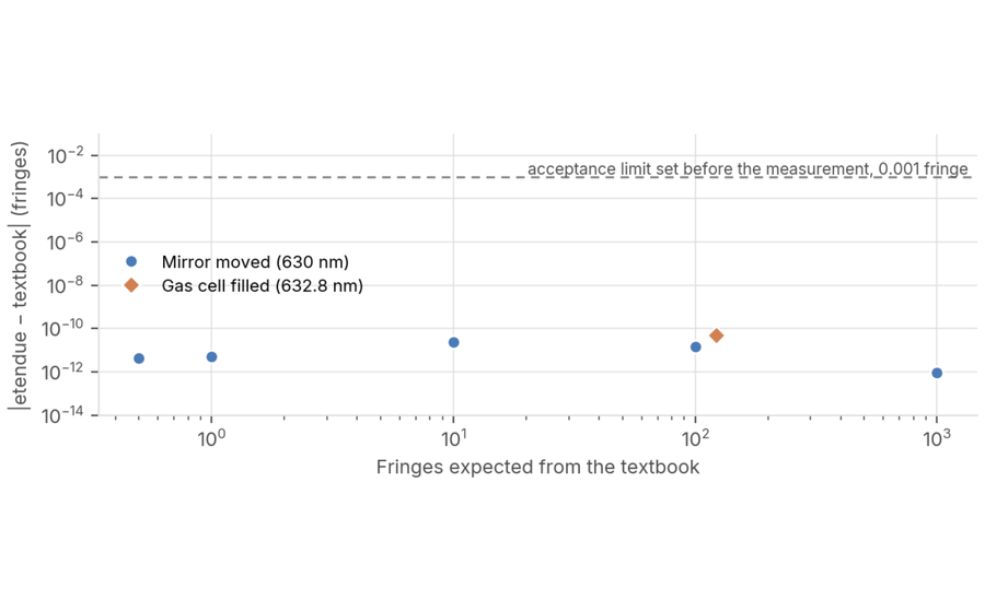
 Path difference and fringe count in a Michelson interferometer
The etendue non-sequential ray tracer compared with the worked examples of OpenStax University Physics, volume 3, section 3.6
How etendue measures up
At every release, we test our AI tools on real specifications and compare our simulation engines with published references. Every result is published, good or bad.
66%
of 1,080 specifications reach their quality target, up from 59% in August 2026.
1,080
real specifications, from ultraviolet to long-wave infrared.
37
designs on target optically, rejected only for their length.
15,691
starting designs built, with up to 5 minutes per specification.
Where the Seed Generator delivers
It is the combination of field and aperture that decides, not either one alone.
Each cell is one combination of focal length, full field of view and aperture, tested in six spectral bands. The number is the share of bands in which the starting design reaches its quality target. Pick an aperture.
1°
5°
15°
35°
65°
100°
1,000
83
50
17
0
0
0
300
83
83
83
83
0
0
100
100
100
100
83
50
17
30
100
100
100
100
83
50
10
100
100
100
100
83
33
3
67
100
100
67
33
33
0%
100% of spectral bands covered
focal length (mm) × full field of view (°)
By spectral band, at f/4
UV39%
Visible69%
NIR69%
SWIR61%
MWIR81%
LWIR78%
Read the grid from corner to corner. A narrow field at f/16 reaches its target in almost every band. At 100° wide open, nothing comes close. The boundary runs diagonally between the two.
What the Seed Generator actually produces
Starting designs, before any optimization.
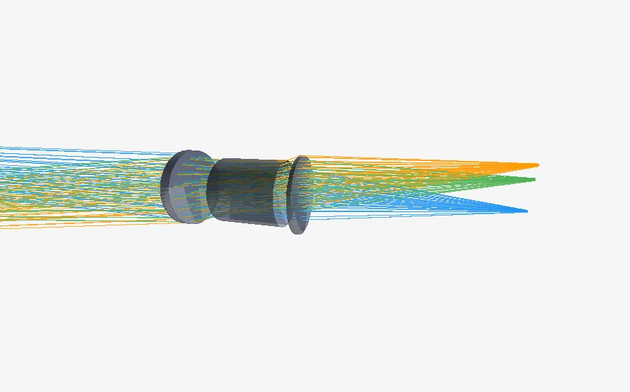
Ultraviolet lens
30 mm · f/4 · 15° field · refractive
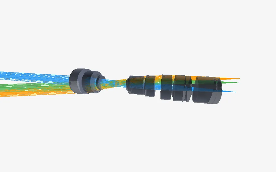
Short-wave infrared lens
30 mm · f/8 · 15° field · refractive
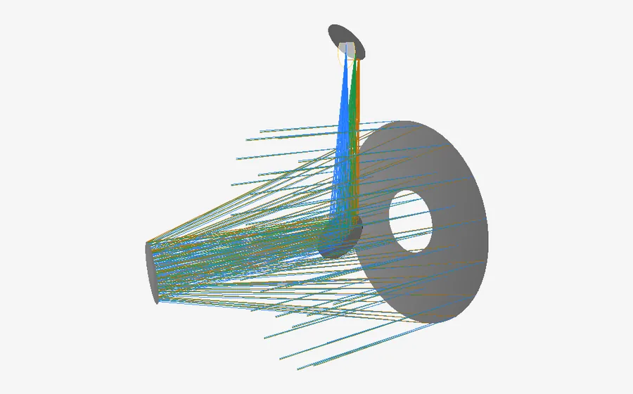
Short-wave infrared telescope
100 mm · f/8 · 1° field · reflective
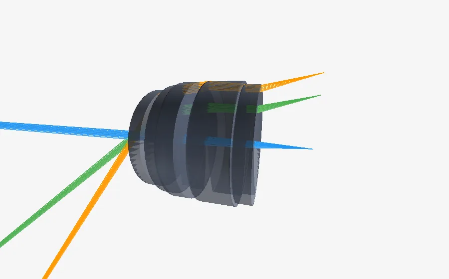
Mid-wave infrared fisheye lens
10 mm · f/8 · 100° field · refractive
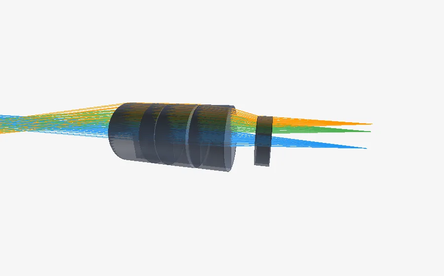
Mid-wave infrared lens
100 mm · f/8 · 15° field · refractive
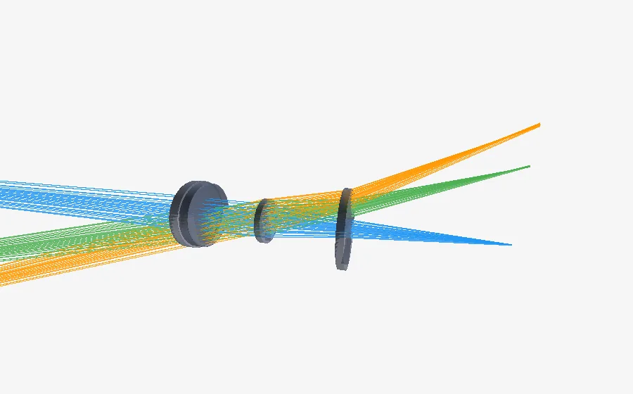
Long-wave infrared lens
30 mm · f/8 · 35° field · refractive
How to read these numbers
1,080 real specifications
Six spectral bands, six focal lengths from 3 to 1,000 mm, six fields of view from 1° to 100°, and five apertures from f/1 to f/16.
One target per specification
A starting design passes when it reaches the quality target set by its specification. Designs that meet the optical target but are too long are counted separately.
Measured at every release
The same specifications are run again at every release, and the results are published: 59% in August 2026, 66% in October 2026.
Explore the full results
The published data behind these numbers, version by version.
The quality of the Seed Generator's starting points, before any optimization, measured on real specifications. Choose a version: depending on the campaign, results are grouped by application domain, with sliders to set your case, or listed specification by specification. Each design gets a single score: 0 is the physical limit, 1 the acceptance threshold.
A.R.G.O.S. explores the optical design space for you.
-
51%
Final design Every requirement met, manufacturing included. Nothing left to do. -
15%
Almost there Image quality within twice the target. It needs tightening. -
13%
Solid starting point Architecture, glasses and size in place; the image is still clearly below target. -
21%
Out of reach in 60 minutes Far from the target, or no usable design.
100 lenses, from UV to thermal infrared · 60 minutes of design each, no intervention · How we measure
Explore the full results
Each dot is a lens designed by A.R.G.O.S.: the closer to the center, the closer to its target; click a dot to open its design.
How to read these numbers
The specification grid
100 imaging lenses on a grid: six bands from ultraviolet to thermal infrared, focal lengths from 3 to 1000 mm, fields from 1° to 100°, apertures from f/1 to f/16. The target: a spot within twice the diffraction limit. Every design gets the same design time.
Distance to target
For each specification, the worst-met requirement of the delivered design, divided by its target. The card shows the geometric mean over the set. 1 × = target reached, smaller is better. A specification with no usable design has no distance: it is counted separately and left out of the average.
All requirements met
The number of specifications whose delivered design meets every requirement, optical quality and manufacturing included.
Ray tracing engine
Follow the light wherever your system sends it.
Each engine is checked against published systems (patents, papers, measurements). The full studies are online.
The engine traces real rays according to the laws of geometrical optics: refraction, reflection, ray splitting at glass surfaces, scattering, diffraction by gratings.
Sequential mode
Rays cross the surfaces in a fixed order. This is the standard mode for lenses and imaging systems.
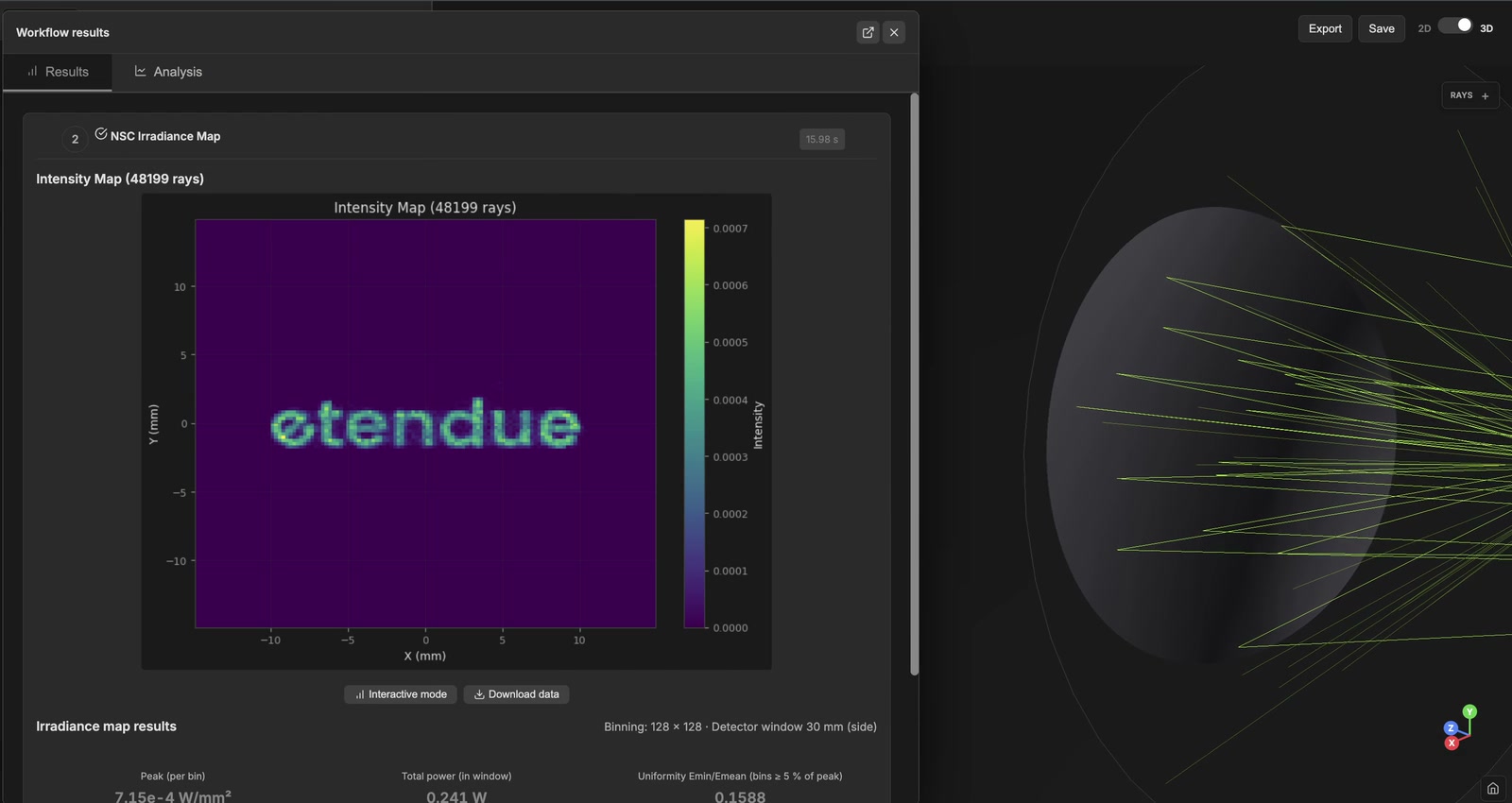
Non-sequential mode
Each ray finds its own path: multiple reflections, a reflected and a transmitted ray at every glass surface, surface and volume scattering, CAD meshes for the mechanics. Hundreds of millions of rays per scene.
One model
A sequential design becomes a non-sequential scene without being rebuilt: you design in sequential mode, then check ghosts and stray light. On a grating system, each diffraction order you choose is traced through the same optics.
Analyses and tools
Sequential analyses
Aberration Analysis
Characterizes the aberrations of a sequential system: Seidel sums, third-order aberrations, Zernike coefficients of the wavefront, ray fans, field curvature and distortion.
- Ray tracing
Chromatic Aberration Analysis
Longitudinal (axial) and lateral (transverse) chromatic aberration of a polychromatic system, angular dispersion of afocal systems and prisms, and overlap of diffraction orders in spectrometers.
- Ray tracing
Distortion Analysis
Measures the geometric distortion of a sequential system: percent or absolute distortion against field angle (f-tan or f-theta), a distorted grid compared with the ideal grid, or the chief-ray angle on the image and object sides (telecentricity).
- Ray tracing
Ghost Focus Generator
Lists every double-reflection ghost of a sequential system, gives the focus, the working F-number and the spot size of each on the image surface, and ranks them from the most to the least visible.
- Ray tracing
Irradiance Analysis
Computes the irradiance map (power per unit area) on the detector surface of a sequential system, for a rectangular or circular detector window that you size.
- Ray tracing
MTF Analysis
Modulation transfer function: how much contrast the system transfers from object to image at each spatial frequency, tangential and sagittal, compared with the diffraction limit, with an optional through-focus curve.
- Ray tracing
- Diffraction
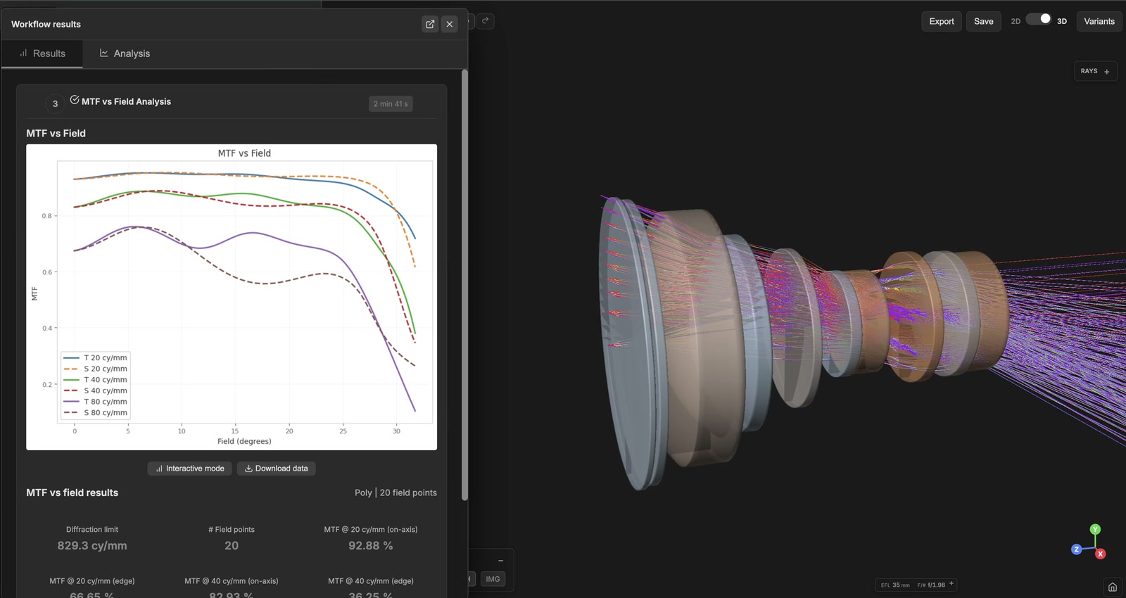
MTF vs Field Analysis
Contrast (MTF) at a few target spatial frequencies across the whole field, from the axis to the maximum field, with tangential (solid) and sagittal (dashed) curves for each frequency.
- Ray tracing
- Diffraction
OPD Analysis
Optical path difference: map of the wavefront error across the exit pupil for each field and wavelength, with its RMS and peak-to-valley values in waves.
- Ray tracing
Polarization Analysis (Sequential)
Follows a polarized beam through a sequential lens system with Jones calculus: transmission with Fresnel losses, Jones matrix, Stokes parameters, and optional maps over the pupil of proper retardance, slow axis, diattenuation, skew aberration and polarization ellipses.
- Ray tracing
Energy in a cone
Share of the power of a Lambertian emitting face (LED or similar source) that leaves the system within a half angle of the image-plane normal, with the capture, the collimation and the curve of that share against the angle.
- Ray tracing
PSF Analysis
Point spread function: the image of a point source formed by the system, including diffraction, with the Strehl ratio, cross-sections and encircled energy, by FFT, Huygens-Fresnel or coherent segmented-pupil methods.
- Ray tracing
- Diffraction
RMS vs Field & Wavelength
Builds a matrix of RMS spot size or RMS wavefront error for every field point and every wavelength of the system, with an optional pass/fail check against a threshold and a heat map.
- Ray tracing
Spot Diagram
Where the rays from the entrance pupil land in the image plane, for each field and wavelength, with the RMS and geometric spot radii compared with the Airy ellipse of that field, at the field's own working F-number.
- Ray tracing
Athermal Analysis
Computes the focus shift of a sequential system across an operating temperature range, from glass index change and expansion of glass and housing, and compares it with the depth of focus to give a pass or fail verdict.
- Ray tracing
- Thermal
Vignetting Analysis
Relative illumination across the image field, with its natural (cos⁴) and mechanical (aperture clipping) contributions, the edge illumination and the on-axis pupil transmission.
- Ray tracing
Image Simulation
Shows how a test chart or one of your images looks on the detector of a sequential system: by convolution with a field-variant PSF (diffraction included), or by tracing rays from every scene pixel (one point can give several images, as through a microlens array).
- Ray tracing
- Diffraction
Chief Ray Solve
Traces a real chief ray through the system and moves the image plane (decenter, tilt, distance) so that the chief ray lands at a target height, like the chief ray solve of common design software.
- Ray tracing
Optimization and tolerancing
Optimization
Optimises the current sequential system against a merit function from the Merit Function Editor: local least-squares (TRF, Dogbox), gradient (L-BFGS-B, BFGS), hard-constraint (SLSQP, trust-constr), derivative-free (Powell) and global (Differential Evolution, Dual Annealing, Brute force) methods.
- Ray tracing
Tolerancing
Statistical tolerancing: perturb the design within manufacturing tolerances, track performance metrics across random draws, and estimate the yield. Monte Carlo (exact) or analytic (fast, linearised wavefront model).
- Ray tracing
Non-sequential analyses
NSC Chromatic Aberration
Measures how the image moves with colour in a non-sequential scene: best-focus shift along the axis and centroid shift across the field, one trace per selected wavelength.
- Ray tracing
NSC Encircled Energy
Radius, centred on the beam centroid or on the axis, that contains 50, 80 and 90 percent of the power reaching a detector in a non-sequential scene.
- Ray tracing
NSC Far-Field (Angular)
Angular intensity distribution at infinity of a non-sequential scene: ray directions binned in polar and azimuthal angle, for beam patterns, BSDF and angular stray-light spread.
- Ray tracing
NS photometry
Intensity distribution in candelas of the light escaping a non-sequential scene, on a horizontal and vertical angular grid, with optional regulation screening and CSV, IES or EULUMDAT export.
- Ray tracing
Illumination optimization
Shape the irradiance on an existing detector of your complete non-sequential system: design or refine a freeform mirror, or set the relative flux of each emitter of a pixel-matrix source to flatten a line. Judged by a full ray trace; the result is applied to the scene.
- Ray tracing
NSC Flux Budget
Radiometric audit of a non-sequential scene: source power, power reaching the detector, throughput, power absorbed on each face, and étendue estimates.
- Ray tracing
NSC Irradiance Map
Two-dimensional map of the power striking a detector in a non-sequential scene: where the light lands, how uniform it is and how intense the hotspots are.
- Ray tracing
NSC Modulation Transfer Function
Modulation transfer function of a non-sequential scene, from the Fourier transform of a diffraction PSF built on the traced rays: tangential and sagittal curves, MTF50, MTF10 and sensor Nyquist.
- Ray tracing
- Diffraction
NSC Point Spread Function
Diffraction point spread function at a detector of a non-sequential scene, by coherent summation of the traced rays: PSF map, widths at half maximum and peak intensity.
- Ray tracing
- Diffraction
PST Sweep (Point Source Transmittance)
Point source transmittance versus off-axis source angle for a non-sequential scene, split into direct, Fresnel ghost and scattered light, with the exclusion angle for a threshold.
- Ray tracing
NSC Spot Diagram
Spot diagram of the rays that reach a detector in a non-sequential scene: RMS and geometric radius, centroid, ghost rays drawn apart and the share of the spot they bring.
- Ray tracing
NSC Stray Light
Splits the light reaching the detector of a non-sequential scene into direct, Fresnel ghost and scattered parts, ranks ghost and scatter paths, and gives the angular far-field of the scattered light.
- Ray tracing
Polarization Analysis
Non-sequential polarization analysis on the GPU engine: output polarization state, Stokes parameters, degree of polarization, phase retardance and extinction ratio of the rays that reach the detector.
- Ray tracing
Tolerancing (non-sequential)
Statistical tolerance analysis of a non-sequential scene: components are moved or reshaped at each draw, the rays are retraced, and metrics are read on detectors.
- Ray tracing
Laser analyses
Laser Beam Propagation
Propagates the laser source of the system through the real sequential layout, folds included: a fast Gaussian caustic, or the wave-optics beam profile at the planes you choose.
- Ray tracing
- Wave optics
Laser Power Budget
Follows where the laser power goes in the system, in watts: detector, other exits, absorbed and stopped. Gives every ghost its power and fluence and names every surface above its damage threshold.
- Ray tracing
Laser Pulse
Follows a femtosecond pulse through the real system: dispersion of each element and cumulated, output duration and shape, pulse-front delay across the pupil, pulse-front tilt and nonlinear phase.
- Ray tracing
- Wave optics
Freeform Beam Shaper
Designs the element that turns a Gaussian laser beam into a target irradiance: square, rectangle, disk, ring, polygon, super-Gaussian or a drawn shape. Either a freeform surface designed inside the loaded sequential system, or a phase mask for a spatial light modulator (SLM).
- Ray tracing
- Wave optics
Surfaces and components you can model
Sequential mode
Basic
- Standard
- Plane
- Paraxial (thin lens)
Conic variants
- Biconic
- Toroidal
Aspheric
- Even asphere
- Odd asphere
Freeform
- Polynomial
- Zernike
- NURBS
- Chebyshev
- Forbes Q2D
- Forbes Qbfs
Advanced
- Grid sag
- Lens array
- Metasurface (metalens)
- Pixellated phase mask
- Pixellated phase mirror (SLM)
- Segmented
Prisms
- Prism
Gratings
- Grating
Non-sequential mode
Sources
- Parallel ray source
- Hexagonal ray source
- Gausslet source
- Broadband Gausslet source
- Confocal ray source
- Point source
- Extended source
- Rayfile source
- Goniometric source
Lenses
- Plano-convex lens
- Plano-concave lens
- Biconvex lens
Mirrors
- PEC mirror
- Coated mirror
Beamsplitters
- Beamsplitter
- Polarizing beamsplitter
Prisms
- Prism
Apertures
- Circular aperture
- Rectangular aperture
Gratings
- Linear grating
- Radial grating
- VPH grating
Detectors
- Ray capture plane
- E-field plane
- Spot diagram
- Intensity map
Mechanical
- Baffle plate
- Tube
- Box enclosure
- Vane stack
- Imported mesh
Media
- Participating medium
Use cases
Path difference and fringe count in a Michelson interferometer
The etendue non-sequential ray tracer compared with the worked examples of OpenStax University Physics, volume 3, section 3.6
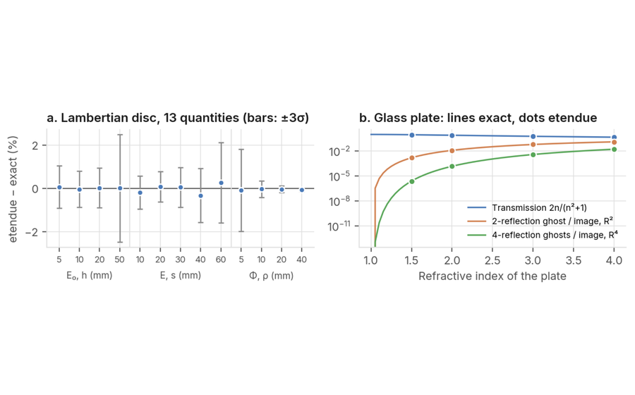 Irradiance of a Lambertian source and ghost reflections of a glass plate
The etendue non-sequential ray tracer compared with exact radiometric view factors and with the Fresnel reflectance at normal incidence
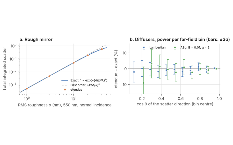 Total integrated scatter of a rough mirror, and Lambertian and ABg diffusers
The etendue non-sequential ray tracer compared with the Davies and Bennett-Porteus scatter law, the Lambertian view factors and the integral of the ABg model
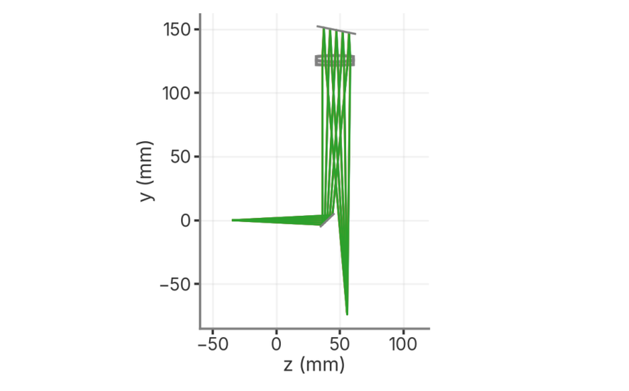 Ray tracing of a 600 lines/mm Littrow spectrograph against the grating equation
Plane reflection grating, 200 mm achromatic doublet used twice, 625 to 680 nm
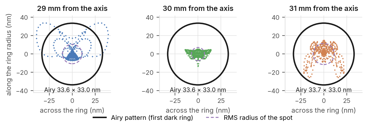 Six-mirror EUV projection objective: aperture on the ring field, image quality and light budget
Four-times reduction, image-side NA 0.25, 13.4 nm, six aspheric mirrors after patent US 6,188,513
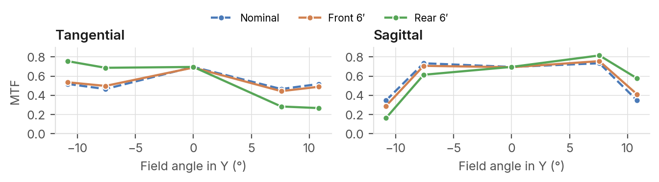 Image contrast of a 36 mm f/2 imaging lens with imposed group tilts
Eleven-lens objective of patent US 8,879,901, three lens groups, 12 variants, polychromatic MTF at 50 cycles/mm
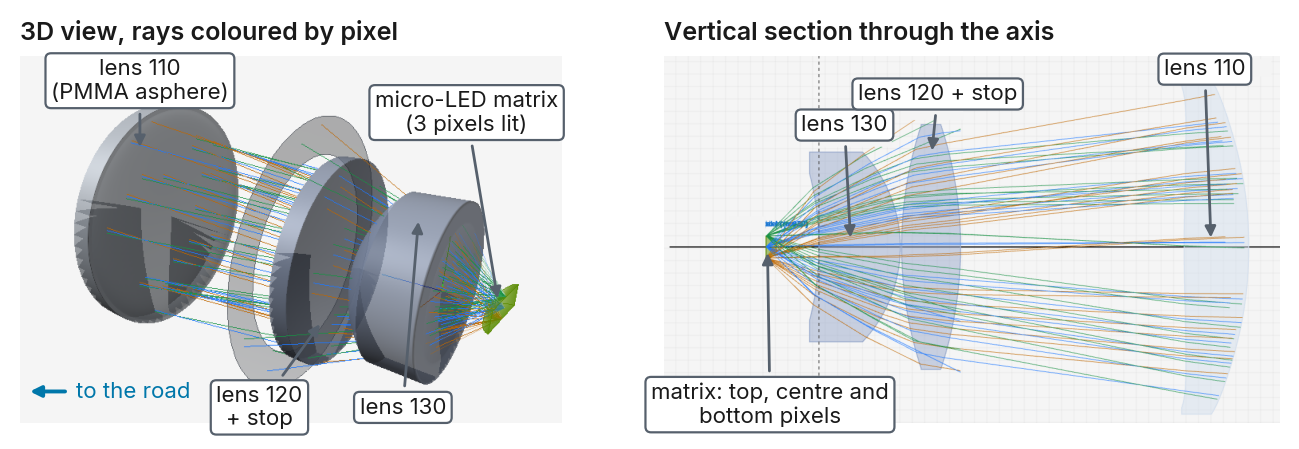
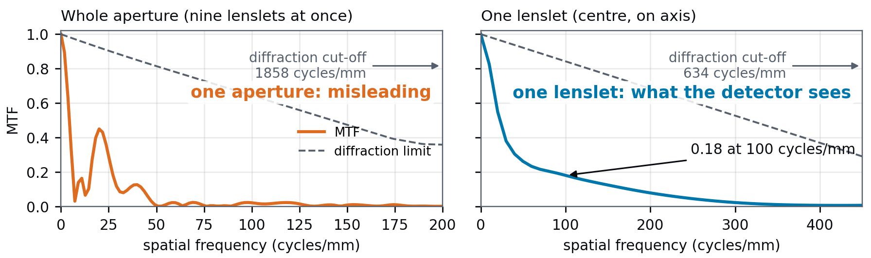 Designing a microlens array imager: per-lenslet image quality, crosstalk and manufacturing data
3 × 3 lens array, 1 mm pitch, re-imaged onto a detector by a 1:1 relay at 550 nm
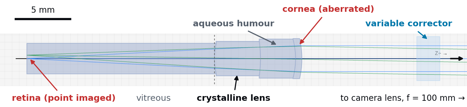 Correcting the aberrations of the eye in a retinal imager with a variable Zernike corrector
Schematic eye with an aberrated cornea, 3 mm pupil, 840 nm; corrector plate with 12 Zernike terms; ICNIRP exposure check
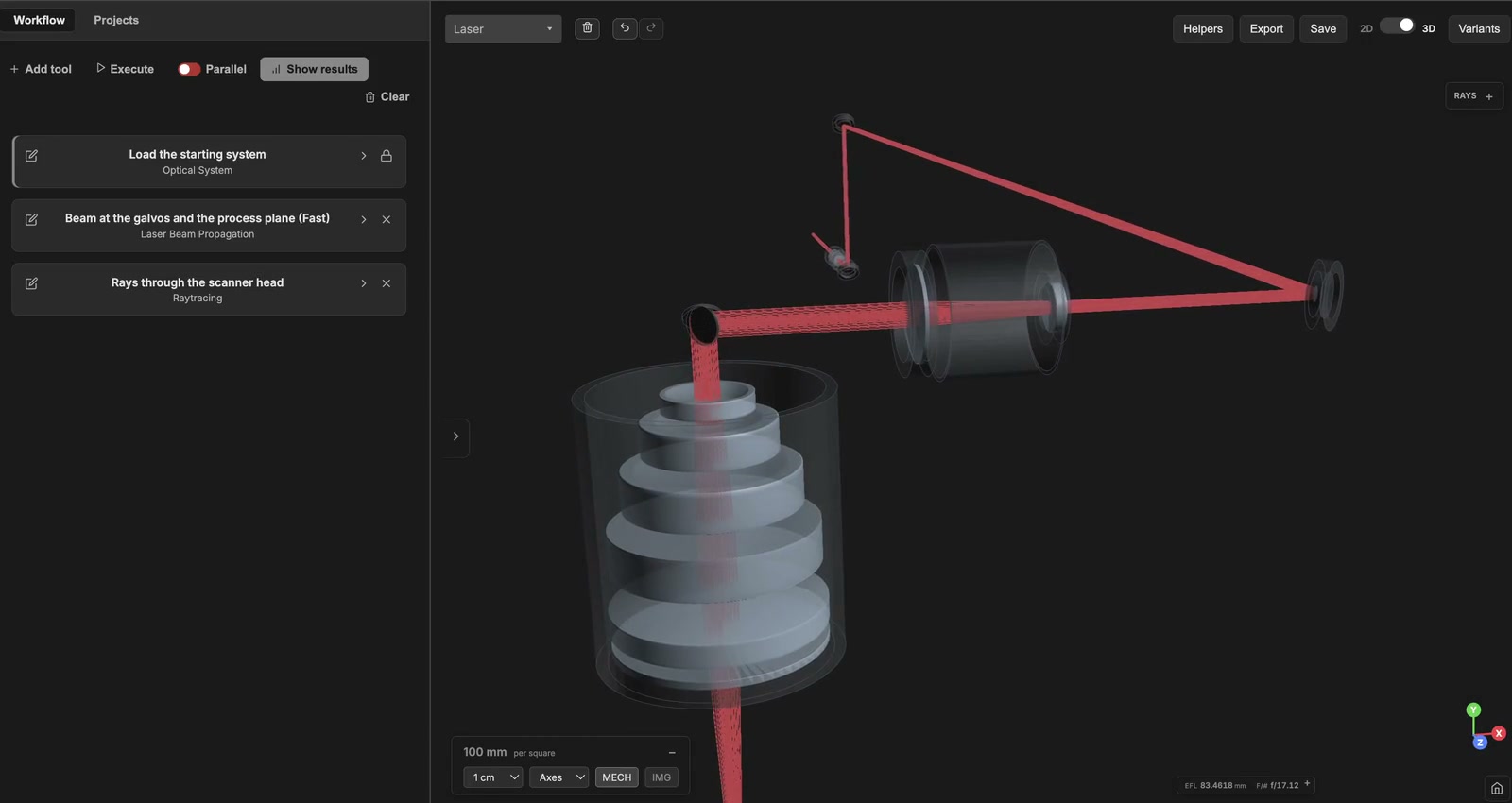
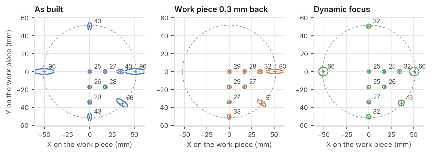 Spot size and shape across the field of a galvo scanner with a telecentric F-theta lens
80 W femtosecond laser at 1030 nm, two-axis galvo head, ±18° scan field
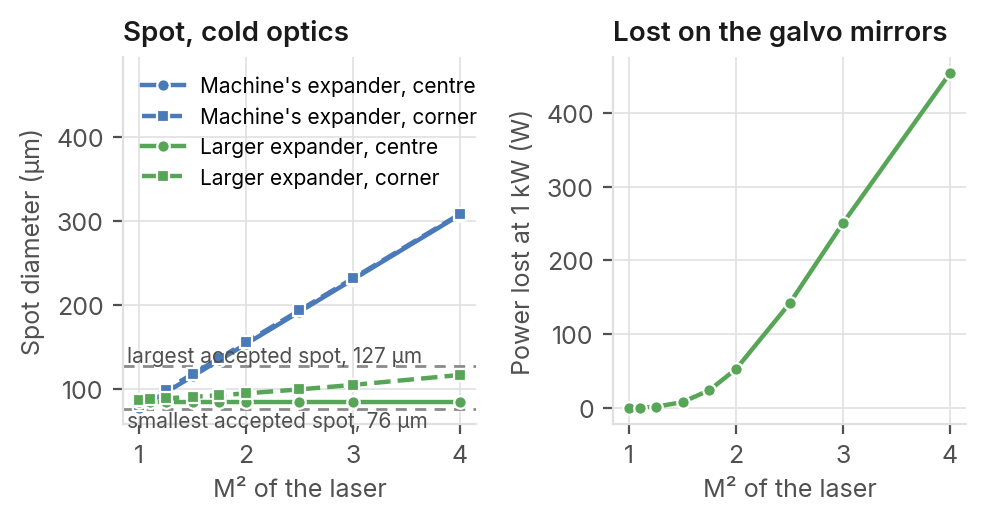 Integrating lower-quality fibre lasers in an LPBF machine: spot size at the powder bed
1 kW fibre laser at 1070 nm, two-axis galvo head and F-theta lens, 250 × 250 mm build plate
Physical optics engine
Where geometrical optics is no longer enough.
Each engine is checked against published systems (patents, papers, measurements). The full studies are online.
The physical optics engine computes what geometrical optics alone cannot: diffraction, interference and the partial coherence of a scalar wave field.
It starts from your geometric model. PSF, MTF, encircled energy and Strehl ratio are computed from the real wavefront that the ray trace gives in the exit pupil, by Fourier transform or by direct Huygens summation. A laser beam is propagated as a complex field sampled on a grid, through the real surfaces of your system, by angular spectrum or Fresnel propagation. You move from ray tracing to wave optics when the question calls for it, without modeling the system twice.
Rays and waves share one and the same model.
Analyses and tools
Sequential analyses
Metasurface Lens
Builds the metasurface lens of the system from its pillar library and compares it, at the image plane, with the ideal lens: focusing efficiency, FWHM, Strehl ratio, background and crosstalk between beams.
- Wave optics
MTF Analysis
Modulation transfer function: how much contrast the system transfers from object to image at each spatial frequency, tangential and sagittal, compared with the diffraction limit, with an optional through-focus curve.
- Ray tracing
- Diffraction
MTF vs Field Analysis
Contrast (MTF) at a few target spatial frequencies across the whole field, from the axis to the maximum field, with tangential (solid) and sagittal (dashed) curves for each frequency.
- Ray tracing
- Diffraction
PSF Analysis
Point spread function: the image of a point source formed by the system, including diffraction, with the Strehl ratio, cross-sections and encircled energy, by FFT, Huygens-Fresnel or coherent segmented-pupil methods.
- Ray tracing
- Diffraction
Image Simulation
Shows how a test chart or one of your images looks on the detector of a sequential system: by convolution with a field-variant PSF (diffraction included), or by tracing rays from every scene pixel (one point can give several images, as through a microlens array).
- Ray tracing
- Diffraction
Non-sequential analyses
NSC Modulation Transfer Function
Modulation transfer function of a non-sequential scene, from the Fourier transform of a diffraction PSF built on the traced rays: tangential and sagittal curves, MTF50, MTF10 and sensor Nyquist.
- Ray tracing
- Diffraction
NSC Point Spread Function
Diffraction point spread function at a detector of a non-sequential scene, by coherent summation of the traced rays: PSF map, widths at half maximum and peak intensity.
- Ray tracing
- Diffraction
Laser analyses
Laser Beam Propagation
Propagates the laser source of the system through the real sequential layout, folds included: a fast Gaussian caustic, or the wave-optics beam profile at the planes you choose.
- Ray tracing
- Wave optics
Laser Pulse
Follows a femtosecond pulse through the real system: dispersion of each element and cumulated, output duration and shape, pulse-front delay across the pupil, pulse-front tilt and nonlinear phase.
- Ray tracing
- Wave optics
Laser Thermal Lens
Follows the thermal lens that a continuous laser, or a pulsed one at its average power, creates in the system: heated glasses and absorbing mirrors, changed optics, new beam, until nothing moves. Asks for no input. Gives the focus shift, the waist change and the heat to remove.
- Wave optics
- Thermal
Nonlinear effects (Kerr, absorption)
Computes the index change (optical Kerr effect) and the multiphoton absorption the laser itself creates in every glass it crosses, at the peak power of the source, and attaches the map to the system.
- Wave optics
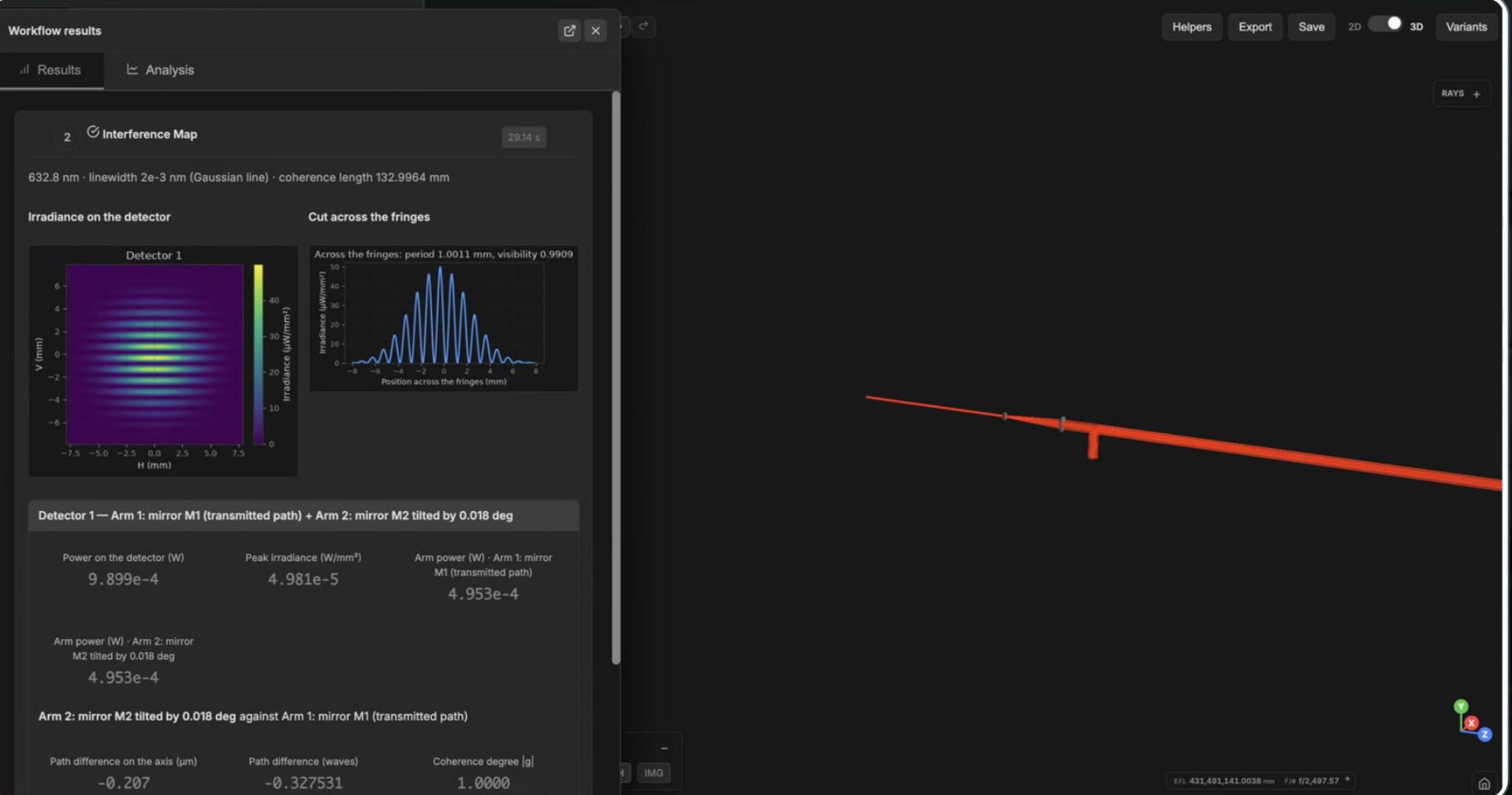
Interference Map
Fringes of an interferometer modelled with one configuration per arm: each arm is propagated by wave optics to the detector and the fields of the arms are added, with the coherence of the laser line.
- Wave optics
Line Homogenizer
Line made by a homogenizer of two cylindrical lens arrays and a Fourier lens with a partially coherent laser: length, contrast, uniformity, edges and profile.
- Wave optics
Waist Fit from Measurements
Reconstructs the waist radius, waist position, M² and Rayleigh range of a Gaussian beam from beam sizes recorded at several positions along the axis. Laser mode step: it recalibrates the laser source of the system.
- Wave optics
Magic Waist Optimization
Moves the lenses of the system in place to put the target waist on the image plane, on both axes. The laser source is read from the system.
- Wave optics
Freeform Beam Shaper
Designs the element that turns a Gaussian laser beam into a target irradiance: square, rectangle, disk, ring, polygon, super-Gaussian or a drawn shape. Either a freeform surface designed inside the loaded sequential system, or a phase mask for a spatial light modulator (SLM).
- Ray tracing
- Wave optics
Laser calculators
4F Telescope
Sizes a two-lens afocal relay (4F system): finds the focal lengths, the magnification and the lens spacing from beam diameters, a target magnification or two known focal lengths.
- Wave optics
Cavity Analysis
Designs and analyzes an optical resonator with Gaussian beam optics: stability, TEM00 eigenmode (waist, position, divergence, astigmatism), finesse and free spectral range, and sensitivity to tolerances.
- Wave optics
Fiber Coupling Analysis
Computes the efficiency with which a Gaussian beam couples into a single-mode fiber, from the mismatch between the beam waist and the fiber mode, with the alignment tolerance budgets for lateral, angular and axial errors.
- Wave optics
Gaussian Beam Propagation
Propagates a Gaussian beam through free space with Fresnel diffraction and returns the full two-dimensional intensity distribution, peak, total power, centroid and the waist after propagation.
- Wave optics
Use cases
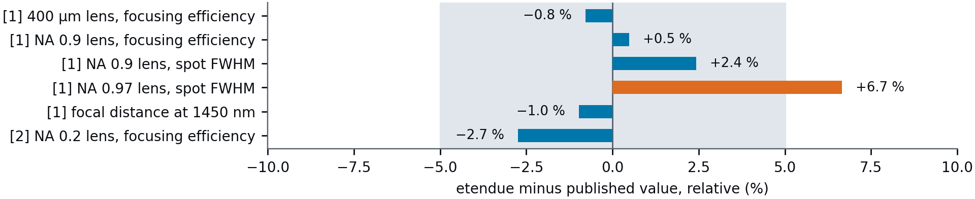 Metalens modelling in etendue reproduces published focusing efficiencies, spot sizes and focal shifts
Two published metalenses recomputed from their nanostructure: amorphous-silicon posts at 1550 nm and silicon-nitride posts at 550 nm
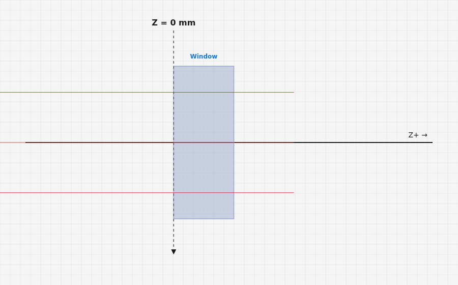 Femtosecond pulse in a glass window
Dispersion, B-integral and Kerr lens against published data
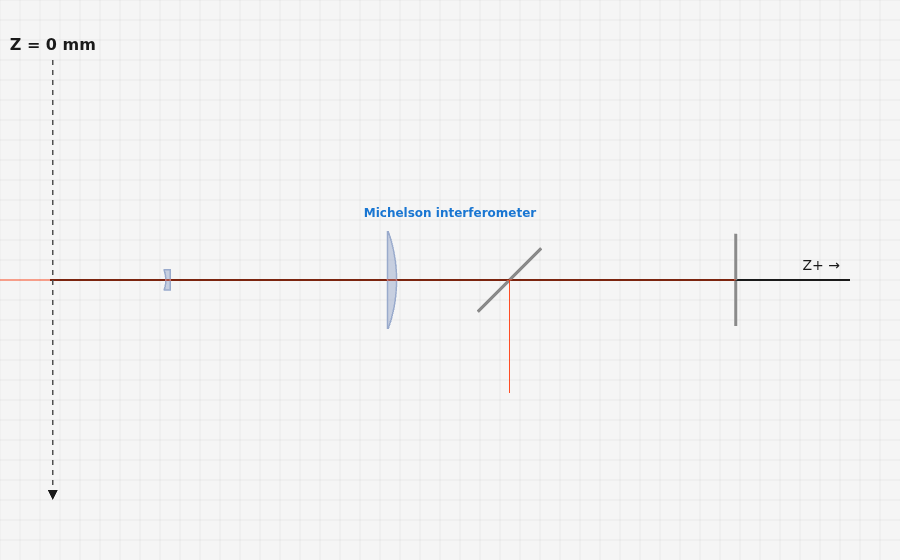 Michelson and Mach-Zehnder interferometers
Fringes, visibility and coherence against textbook results
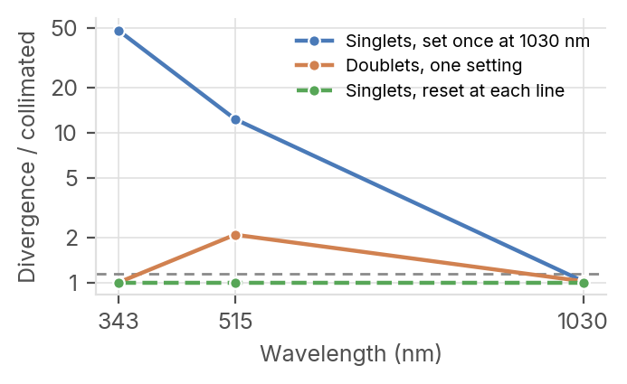 Lens spacing of a 3× beam expander used at 1030, 515 and 343 nm
Fused-silica singlets against CaF2 / fused-silica doublets for the three harmonics of a Yb laser, with the collimation read on the Gaussian beam at each line
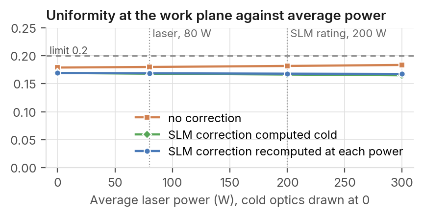 Square top-hat from a femtosecond laser with a phase-only LCOS SLM
80 W femtosecond laser at 1030 nm, 300 µm square top-hat, average power from 0 to 300 W
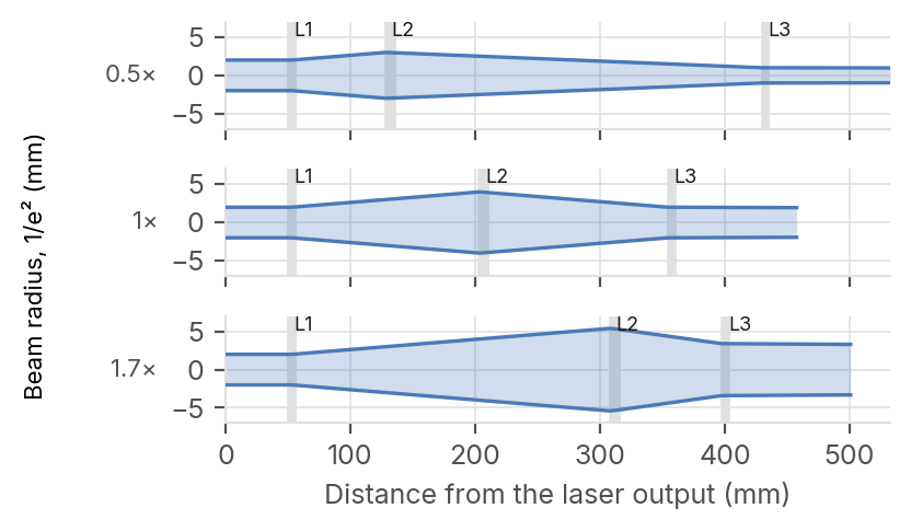 B-integral and pulse duration in a 0.5× to 1.7× ultrafast zoom beam expander
Three-lens Galilean zoom behind a 1030 nm femtosecond laser, 7 variants, pulse propagated through the real system at each position
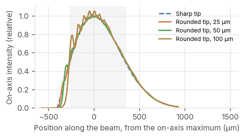 Core size, zone length and axicon tip tolerance of a Bessel beam shaper for glass cutting
Ultrashort-pulse laser at 1030 nm, fused-silica axicon and a reducing telescope, after Balage et al.; wave-optics field computed plane by plane along the Bessel zone
Thermomechanical engine
A system that meets its specification at 20 °C may not meet it at −40 °C or +80 °C.
Each engine is checked against published systems (patents, papers, measurements). The full studies are online.
The thermomechanical engine computes how temperature changes your glasses and mounts, and brings in the deformations from your finite element software.
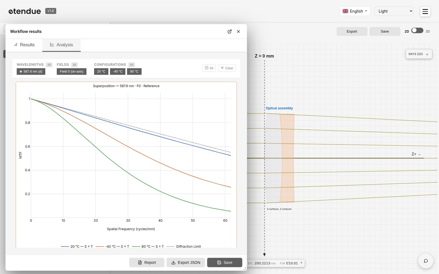
Indices, radii of curvature, thicknesses and air gaps change with temperature, and a thermal gradient between parts is applied part by part. Deformations imported from a finite element analysis are split into rigid-body motion (decenter and tilt) and surface deformation. The effect on image quality is measured with your usual analyses, MTF included.
A design is checked across its whole temperature range, not at a single point. Each temperature is a full simulation of the system rebuilt at that temperature, and the cloud runs them in parallel.
Analyses and tools
Sequential analyses
Athermal Analysis
Computes the focus shift of a sequential system across an operating temperature range, from glass index change and expansion of glass and housing, and compares it with the depth of focus to give a pass or fail verdict.
- Ray tracing
- Thermal
Laser analyses
Laser Thermal Lens
Follows the thermal lens that a continuous laser, or a pulsed one at its average power, creates in the system: heated glasses and absorbing mirrors, changed optics, new beam, until nothing moves. Asks for no input. Gives the focus shift, the waist change and the heat to remove.
- Wave optics
- Thermal
In the optical editor
- Expansion laws per glass and per mount material, and a temperature range for each configuration.
- Thermal gradients between parts, applied part by part.
- Deformations imported from a finite element analysis (CSV or NASTRAN), split into rigid-body motion and surface deformation.
Use cases
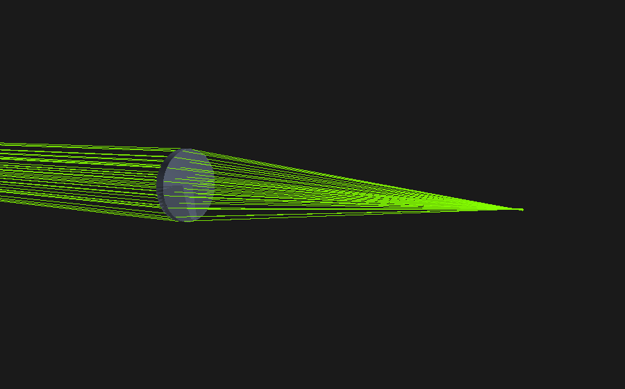 Thermal focus drift of a glass lens, checked against published glass data
N-BK7 plano-convex lens, f = 100 mm at f/4, three wavelengths, −40 to +80 °C, two mount materials
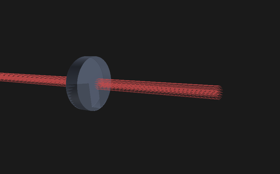 Thermal lens of a laser-heated fused-silica element, checked against analytical solutions
1000 W Gaussian beam at 1064 nm, steady state, heat absorbed in the bulk or in a coating
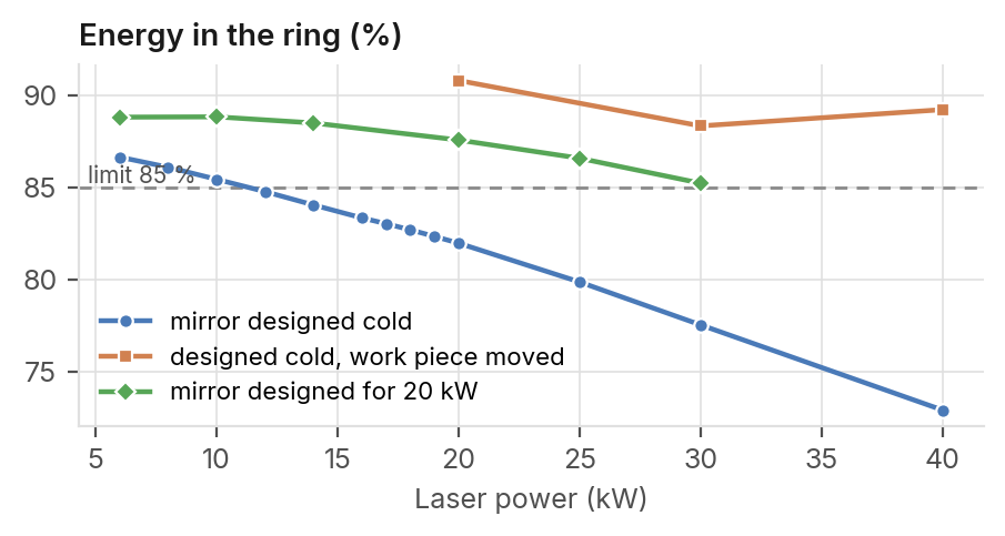 Thermal limits of a freeform ring-shaping head for a multimode fibre laser
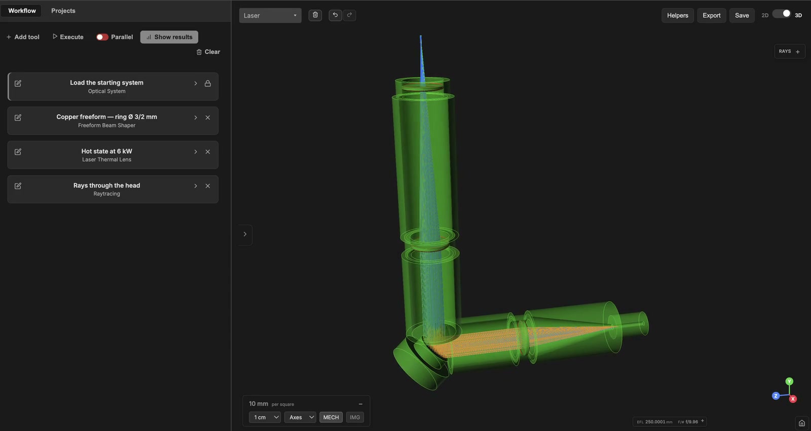
Laser welding head at 1030 nm, ring of 3 / 2 mm diameter, laser power from 6 kW to 40 kW
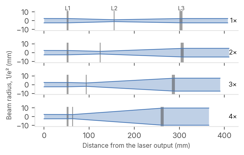 Collimation and thermal lens of a 1×–4× zoom beam expander at 1 kW
Galilean zoom with three fused-silica lenses, four zoom positions optimized together, 1030 nm continuous laser from 100 W to 1 kW