
other
Benchmark Visible Littrow spectrograph
From the optical layout to spectral dispersion
Benchmark Visible Littrow spectrograph
From the optical layout to spectral dispersion
This case study takes you through a visible spectrograph in etendue.io, from opening a ready-to-run project to inspecting its optical path and comparing its spectral dispersion with a published observation.
The system is inspired by the LHIRES III spectrograph. It combines a real achromatic doublet used in double pass with a 600 lines/mm reflection grating, following the architecture described by Shelyak [2].
The objective is to follow the simulation workflow, understand what the displayed results mean, and assess how closely the reconstructed model matches Christian Buil’s November 2006 measurement [1].
Start with the preset and the 2D and 3D views, then read the chromatic analysis. The scientific comparison and its limits follow the same sequence, from dispersion to resolving power.

LHIRES inspired case study | SPEC05 | 25 September 2026
Setting up the system
Open the project library, select the Spectrometers folder, and load “SPEC05 - Littrow réaliste : LHIRES 600 tr/mm, visible”. The setup identifier is littrow_lhires_600tr_realiste.
 The sequential preset contains the folded optical path and both passes through the doublet. Keep its surface positions, tilts and signed propagation distances: on the return pass, the three lens faces are visited in reverse order at the same physical locations
Surface editor with the grating parameters expanded.
| Setting | Value to check |
| Source and wavelengths | Point source; 625, 640, 656.3, 670 and 680 nm; primary 656.3 nm |
| Slit sampling | Object height fields (0, 0), (0, +0.013), (0, −0.013) mm |
| Input cone | Source 34 mm before a Ø3.4 mm launch pupil, giving f/10 |
| Grating | Order +1; 600 lines/mm; period 1.666667 µm; groove orientation 180° |
| Grating aperture | Rectangle; x and y bounds −15 to +15 mm |
| Image area | 8 × 4.6 mm detector window; 9 µm reference pixel pitch |
Run the stored workflow: Load optical system → Ray tracing → Spot diagram → Chromatic dispersion. It uses six rings for ray tracing and the spot diagram, with hexapolar sampling in the spot analysis.
Exploring the simulation views
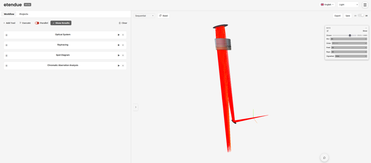
Before reading the numbers, inspect the light path in the 3D view and its alignment in the 2D cut. The input beam reaches the fold mirror, travels towards the doublet and grating, then returns through the same doublet towards the detector.

3D view on the left and 2D cut on the right. The compact group next to the grating is the cemented doublet.
The same lens collimates the input beam and forms the dispersed image on the return path. Its physical faces appear twice in the sequential prescription because the light crosses them twice.
These views help you understand the geometry. To measure the wavelength mapping, use the numerical detector coordinates in the chromatic analysis rather than distances or apparent angles on screen.
Reading the spectral dispersion
In the chromatic analysis, select Angular Dispersion and inspect order +1 at the central field. The table gives the detector position and dispersion for each wavelength, with the detector coordinate set to zero at 656.3 nm.

Chromatic analysis for order +1. Chief ray detector positions run from +3.8508 to −2.9294 mm over the five sampled wavelengths.
To compare with the published 9 µm pixels, multiply the dispersion in nm/mm by 0.009 mm. The displayed exit angle is in mrad and cannot be compared directly with nm/pixel; its negative sign follows the output coordinate convention.
| Quantity | Published reference [1] | Etendue | Difference | ||
| Dispersion | 0.0735 nm/pixel | Band average | 0.072967 nm/pixel | Local value at 656.3 nm | −0.725% |
The calculated dispersion is within 0.73% of the published value. It is obtained from chief ray positions at 656.29 and 656.31 nm. The rounded display value, 8.107 nm/mm, gives 0.072963 nm/pixel; the small difference comes from rounding.
This compares a local model value with a band average. The substitute lens and reconstructed spacings may also contribute to the difference, but their individual contributions have not been isolated. The 3% acceptance criterion was selected for this reconstruction; it is not a measurement uncertainty. Shelyak also lists about 0.074 nm/pixel at Hα for this grating density [2].
Interpreting resolving power
The slit image provides a first geometrical estimate of spectral resolution. Its reconstructed width is 26.535 µm, corresponding to Δλ ≈ 0.215 nm and R = 656.3/Δλ ≈ 3051.
| Quantity | Published reference [1] | Etendue | Difference | ||
| Resolving power R | Approximately 2700 | Instrument result | Approximately 3051 | Slit width only estimate | +13.0% |
These figures use different definitions. A comparison with the observed instrument needs a line profile that includes optical aberrations, diffraction, slit illumination and pixel response. Those effects can broaden a line, but they have not been shown to explain the entire 13% difference. Total instrument resolution is therefore not validated.
Conclusion
The case takes the user from a stored optical setup to an interpretable spectral result. Its strongest experimental comparison is dispersion: the calculated value agrees with the published LHIRES III observation to within 0.73%.
This supports the reconstruction as a geometrical validation case. It does not establish an exact replica of the commercial instrument or validate its total resolving power.
System prescription and reference data
The model follows the LHIRES III architecture described by Shelyak [2]. Since the cited references do not establish the original lens prescription, it uses the documented Edmund Optics 45-415 doublet [3].
| Parameter | Reference or chosen value | Origin |
| Operating conditions | 600 lines/mm; f/10 input; 26 µm slit; 9 µm pixels; 625 to 680 nm | Buil [1] |
| Optical architecture | One Ø30 mm, 200 mm focal length doublet used for collimation and imaging | Shelyak [2] |
| Substitute doublet | N-BK7 / N-SF5; 5.0 / 2.5 mm centre thicknesses; Ø29 mm clear aperture | Edmund [3] |
| Signed surface radii | +123.77 / −89.22 / −259.43 mm in the catalogue direction; f = 200 mm at 587.6 nm | Edmund [3] |
| Finite component sizes | 10 × 14.14 mm fold mirror; 30 × 30 mm grating; 8 × 4.6 mm detector window | Reconstruction |
Additional mechanical inspiration comes from LHIRES 2 [4], including the 74 mm slit-to-fold spacing. Other reconstructed dimensions are a nominal 20 mm lens-to-grating gap and a 6 mm separation offset.
The full doublet and detector were positioned before tracing to collimate and focus at 656.3 nm. No optical surface is subsequently centred on ray impacts.
Sources
[1] Christian Buil LHIRES III spectrograph test with a 600 lines/mm grating November 2006
[2] Shelyak Instruments Lhires III User Guide DC0004A pages 6 and 7 December 2006
[3] Edmund Optics Drawing 45415 30 mm diameter 200 mm focal length achromatic doublet
[4] ARAS Statut technique du spectrographe LHIRES2 figures 4 and 5 November 2004
