Benchmark: Smartphone lens part 1

Benchmark: Smartphone lens part 1

Asphere spot diagram & MTF

This case study is inspired by the Youtube video Smartphone Camera Lens Design: A Patent Study by Stephen Remillard.

The objective of this study is to compare different metrics simulated in Etendue with those from the reference software described in the source material.

Key results: Across all evaluated metrics — Field Curvature, Distortion, MTF vs. Field, and Diffraction MTF — Etendue demonstrates strong agreement with the reference software. Spot diagram metrics show an average deviation of 4%, while MTF profiles are visually identical, confirming Etendue as a reliable tool for optical system analysis.

System prescription:

The simulated setup is a patented^[1] design for a smartphone camera. It’s notably made of aspheric lenses as shown is the table below:

And the coefficients are listed in this table:

Simulation results:

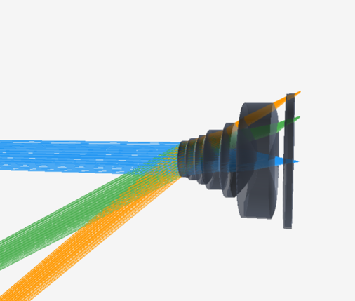
Before analyzing the simulated values, an initial visual check confirms that the system has been correctly reconstructed by the AI using screenshots from the reference material:

2D cut

3D view

Spot diagrams:

Looking at the spot diagrams in etendue and the reference software, we can also confirm that spot diagrams have similar profiles:

And a closer look at the numbers gives a 4% average error:

MTF analysis

In his video, S. Remillard also discusses in length the MTF of the system, let’s compare reference plots against etendue’s ones:

Both plots show the same fundamental behavior: MTF starting at 1.0 on-axis and decreasing monotonically with spatial frequency, with a clear degradation at larger field angles. The relative ranking of field positions (on-axis best, full field worst) is fully consistent between the two tools.

MTF vs field

Both plots show the same general behavior: MTF decreasing with field angle, with characteristic oscillations around 15–20° and 27–30°, and a consistent T/S separation across all spatial frequencies. The ranking of frequency curves (higher MTF at lower lp/mm) is well preserved.

Field curvature :

A visual examination of both plots reveals similar profiles; small deviations point to either a diverging ray tracing model at wide fields or heavier smoothing of the output data.

*Units in µm.

Distortion F(than(theta)

Both plots are in excellent agreement. The S-curve shape, amplitude (~1.9% at full field), zero-crossing location, and overall field behavior are fully consistent between the two tools. Chromatic separation between the three wavelengths is equally tight in both cases.

Conclusion:

Analyzed metrics are similar, demonstrating Etendue’s core engine reliability and precision.

The workflow in Etendue is fast and easy to set up, largely thanks to the AI assistant, which successfully reconstructed the system from scratch by analyzing screenshots from the source material.

The next case study on this system will focus on tolerancing and optimization.

1. Chen, Chun-Shan, Tsung-Han Tsai, and Ming-Ta Chou. "Optical image lens system." U.S. Patent No. 11,561,375. Jan. 24, 2023 ↑